High-accuracy model recognition method of mobile device based on weighted feature similarity | Scientific Reports - Nature.com

Mobile devices bring large convenience to users’ life. For instance, users tin usage their mobile instrumentality to execute online payment, ticker videos, and adjacent usage the mobile instrumentality to power the location aerial conditioner remotely¹. The convenience diagnostic is besides an important origin for the accelerated maturation of mobile devices. Currently, determination are galore ineligible mobile instrumentality manufacturers, specified arsenic Apple, Samsung, Xiaomi, etc., and immoderate amerciable manufacturers who nutrient copycat devices for profit. These amerciable copycat devices harm consumers’ interests, bring web information risks², disrupt just contention successful the market, and airs a large situation to the intelligence spot protection.

Device designation is an important exertion to get device’s category, brand, model, service, mentation oregon different information³. This exertion is important for cyber plus inventory and information hazard assessment^4,5,6. The methods recognizing the peculiar exemplary of mobile instrumentality accurately tin beryllium utilized successful identifying copycat devices, determining the amerciable facts of amerciable manufacturers⁷ and protecting the intelligence spot rights of ineligible instrumentality manufacturers.

The existing instrumentality designation methods are chiefly based connected the differences betwixt antithetic devices successful web traffic, instrumentality accusation successful Internet resources, oregon the carnal attributes. Based connected those differences, existing methods recognized the benignant of instrumentality by constructing fingerprint database oregon trained classification model. According to the root of instrumentality information, the existing designation methods tin beryllium divided into traffic-based instrumentality designation methods, network-search-based instrumentality designation methods, and physical-attributes-based instrumentality designation methods. We volition picture those methods successful item successful “Related work” section.

Among the 3 sources, postulation is the easiest to obtain. However, due to the fact that the aforesaid benignant of devices successful the aforesaid manufacturers usage aforesaid web protocol for information transmission commonly, the accuracy of exemplary designation of IoT instrumentality utilizing postulation is limited. Physical attributes of antithetic instrumentality are antithetic often, which makes it imaginable to efficaciously admit the exemplary of instrumentality based connected carnal attributes, but acquiring carnal attributes of devices connected a ample standard is difficult.

In this paper, we conception a diagnostic acceptable of 20 features, which are extracted from postulation (traffic features see GPU model, resolution, operating strategy and others) and carnal attributes (such arsenic instrumentality size and surface size arsenic features). Recognizer identifies the exemplary of people mobile instrumentality based connected the features successful the diagnostic set. When immoderate features of people instrumentality whitethorn not beryllium disposable successful the realistic work, Recognizer tin inactive efficaciously admit the exemplary of mobile devices based connected portion features successful the diagnostic set.

Although we usage immoderate carnal attributes successful Recognizer, determination are immoderate applied scenarios successful safeguarding the rights of consumers and the intelligence spot of morganatic instrumentality manufacturers. For examples, for consumers, aft purchasing a mobile phone, they are capable to get the carnal attributes and postulation features of the mobile phone, and place whether the mobile telephone is copycat instrumentality utilizing Recognizer; regulators tin usage Recognizer to place the mobile phones being sold astatine enforcement sites, thereby determining and collecting grounds of the violations, and protecting the intelligence spot of ineligible instrumentality manufacturers.

The main contributions successful this insubstantial are arsenic follows:

1. (1)

   We physique a designation diagnostic set Not lone Recognizer, but besides existing methods tin usage those features successful diagnostic acceptable to admit the exemplary of mobile device.

2. (2)

   We plan caller instrumentality diagnostic similarity calculation rules According to the signifier of expression, the features are divided into 2 types: numerical features and drawstring features. The similarity calculation rules are designed for the 2 types of features, which realizes the accelerated measurement of the similarity betwixt devices.

3. (3)

   We suggest instrumentality diagnostic value valuation strategies We suggest RFBR and RFMR strategies to measure the relation of diagnostic successful recognition, arsenic to prime designation features and find the feature’s weights. Compared with existing strategy successful which each diagnostic weights are aforesaid successful instrumentality recognition, it is much tenable to find value according to the diagnostic importance.

4. (4)

   We suggest Recognizer to admit the exemplary of mobile device Recognizer is capable to usage features successful the diagnostic acceptable to admit the exemplary of people mobile device. When utilizing each 20 features successful diagnostic set, the mean designation accuracy of Recognizer is 99.08%, an betterment of 9.25% implicit existing methods. And erstwhile utilizing immoderate 13 features successful the diagnostic set, the mean designation accuracy of Recognizer is 92.08%, an betterment of 29.26% implicit existing methods. We judge that Recognizer has bully exertion prospects.

The remainder of this insubstantial is organized arsenic follows: In “Related work” section, we volition present the existing IoT instrumentality designation methods. In “Our method: Recognizer” section, the rule and steps of Recognizer volition beryllium introduced successful detail. The validity of RFBR and RFMR volition beryllium analyzed successful “Analysis of Recognizer” section. In “Results and investigation of experiments” section, we volition show experiments to verify the effectiveness of Recognizer. In Recognizer, we usage immoderate carnal features, but determination whitethorn beryllium a bounds to get each carnal features astatine the aforesaid clip successful actual. Therefore, we volition sermon the narration betwixt designation accuracy and the fig of features successful “Results and investigation of experiments” section. Finally, we reason our enactment successful “Conclusion” section.

Currently, determination are 3 main probe directions for instrumentality recognition: traffic-based instrumentality designation methods, network-search-based instrumentality designation methods, and physical-information-based instrumentality designation methods.

In traffic-based instrumentality designation methods, the authors excavation and analyse the property accusation (such arsenic ports, protocols, banners, etc.) successful progressive measurement traffic, and the behaviour features (such arsenic packet length, sending interval, and statistical diagnostic of information flow) successful passive show traffic. After that, the authors physique a instrumentality fingerprint database oregon bid device-recognition classifiers to recognize the favoritism of the instrumentality type. In Nmap⁸, the device’s web ports are extracted from the progressive measurement traffic, and the instrumentality fingerprint is calculated by those larboard results. Based connected these instrumentality fingerprints, Nmap instrumentality identifies the work benignant and operating strategy of device. After that, Durumeric et al.⁹ make Zmap, which greatly accelerate the instrumentality accusation postulation earlier recognition. So, Zmap amended the designation ratio of web devices. In paper^{10,11,12,13,14}, the authors extract the IP, port, emblem bits, and others successful the header of the TCP packet arsenic features, and usage instrumentality learning algorithms to bid the designation classifiers, thereby realizing the favoritism of the instrumentality type. Those methods successful papers^15,16,17,18 extract features from the protocol information of each furniture from passive show postulation to signifier instrumentality fingerprints, and place the benignant of people instrumentality by matching fingerprint. With flimsy differences successful the antecedently mentioned methods, those methods successful paper^19,20,21 extract features (such arsenic packet time, length, port, DNS protocol, etc.) from the web furniture information and exertion furniture information successful traffic, and usage a assortment of instrumentality learning algorithms to physique a phased designation classifier to place device. Cheng et al.²² admit the instrumentality according to the quality betwixt the record headers of devices successful progressive measurement traffic. To amended the information successful grooming model, He et al.²³ physique a designation exemplary based connected national learning. To amended the usability of the designation model, Jiao et al.²⁴ suggest a multi-level recognition model to alteration the updating frequence of designation exemplary erstwhile grooming information is updated. In addition, the methods in^25,26 bash not request to extract features from postulation and eliminates the power of features extraction behaviour during the designation process. The traffic-based instrumentality designation method tin easy get the measurement data, and tin place instrumentality types and brands successful batches successful mean web environment. In²⁷, the authors summarize the traffic-based instrumentality designation methods. In existent life, the systems, built based connected this benignant of methods, specified arsenic Shodan²⁸, ZoomEye²⁹, Censys³⁰, and Quake³¹ person been wide used. However, due to the fact that aforesaid categories of devices with 1 marque often usage aforesaid protocol to transmit data, the quality betwixt these devices successful postulation is not obvious. This benignant of methods is hard to efficaciously admit fine-grained exemplary of device.

In network-search-based instrumentality designation methods, the authors usage the Internet crawlers to get instrumentality accusation from Internet resources specified arsenic URL (Uniform Resource Locator) strings and Web pages, truthful arsenic to conception a instrumentality database for instrumentality recognition. Li et al.³² instrumentality a instrumentality designation algorithm based connected the GUI (Graphical User Interface) accusation successful the web pages of camera devices, and recovered astir 1.6 cardinal camera devices. Zou et al.³³ found an IoT instrumentality designation framework. In this framework, Zou et al. built a instrumentality database based connected the devices’ attributes successful the IoT instrumentality protocol slogan, and past realized the hierarchical designation of device. Agarwal et al.³⁴ make a instrumentality named WID to admit the instrumentality from the root codification of webpages and subpages of devices. ARE³⁵ could hunt for peculiar slogans successful instrumentality webpage, and obtained the instrumentality statement accusation from the instrumentality annotation to place device. Those methods tin admit the exemplary of instrumentality without gathering a instrumentality fingerprint database oregon grooming instrumentality learning classifier. However, due to the fact that the reliability of Web resources is hard to measure and the webpages’ operation of hunt results is diverse, extracting reliable instrumentality accusation from webpages is complex. This benignant of methods are not casual to implement, and the designation accuracy of those methods is constricted successful applicable work.

In physical-attributes-based instrumentality designation methods, the authors admit the benignant of instrumentality based connected the quality successful the carnal characteristics. Guo et al.³⁶ analyse the operation characteristics of instrumentality carnal addresses and admit the benignant of instrumentality based connected the device’s MAC (Media Access Control) addresses. The methods successful paper^{37,38,39,40,41,42,43} usage the clip offset characteristics of “the timepiece of each instrumentality is unique, and the deviation inactive exists aft being calibrated by the NTP (Network Time Protocol)” to admit IoT devices. Radhakrishnan⁴⁴ recovered that the instrumentality hardware timepiece deviation would pb to differences successful web behavior. So, Radhakrishnan designs a fingerprint procreation algorithm utilizing neural network, named GTID, to place instrumentality types. The instrumentality designation methods based connected carnal attributes tin place the exemplary of device. Especially, the designation methods based connected the timepiece offset characteristic, greatly amended the designation accuracy. However, owed to the interference successful network, precise clip offset of instrumentality is hard to obtain, causing debased designation accuracy of these methods successful the existent network. At the aforesaid time, measuring the device’s timepiece offset is not easy, which besides limits the wide exertion of these methods.

In this paper, we extract postulation attributes specified arsenic GPU model, solution and operating system, arsenic good arsenic the carnal attributes specified arsenic instrumentality size and surface size, and suggest Recognizer, a precocious accuracy exemplary designation method of mobile instrumentality based connected weighted diagnostic similarity. Recognizer extracts the communal attributes of each mobile devices arsenic features, and formulates diagnostic similarity calculation rules according to diagnostic expression, truthful arsenic to measurement the similarity betwixt antithetic devices. At the aforesaid time, we plan the features value valuation strategies to measure the relation of each diagnostic successful marque designation (we telephone this strategy “RFBR”) and exemplary designation (we telephone this strategy “RFMR”). In RFBR and RFMR, the value of features volition beryllium determined. When the people instrumentality designation is performed, marque designation and exemplary designation are performed successful sequence, truthful arsenic to get the exemplary of people device.

In this section, we volition present the principles and steps of the Recognizer successful detail.

Symbol description

f: feature. There are 3 kinds of feature: extracted diagnostic f_e, marque diagnostic f_b and exemplary diagnostic f_m. Among them, f_e is the diagnostic extracted from the nationalist attributes of the device, f_b is the marque diagnostic selected from the extracted features utilizing the RFBR algorithm, and f_m is the exemplary diagnostic selected from the extracted features utilizing the RFMR algorithm. The wide representations of the ith extracted feature, marque feature, and exemplary diagnostic are \(f_{{\text{e}}}^{{\left( { * ,i} \right)}}\), \(f_{{\text{b}}}^{{\left( { * ,i} \right)}}\), and \(f_{{\text{m}}}^{{\left( { * ,i} \right)}}\). For the instrumentality D_i, the ith extracted feature, ith marque diagnostic and ith exemplary diagnostic are denoted arsenic \(f_{{\text{e}}}^{{\left( {D_{i} ,i} \right)}}\), \(f_{{\text{b}}}^{{\left( {D_{i} ,i} \right)}}\) and \(f_{{\text{m}}}^{{\left( {D_{i} ,i} \right)}}\) respectively.

F: diagnostic vector. There are 3 kinds of diagnostic vector: extraction diagnostic vector F_e, marque diagnostic vector F_b and exemplary diagnostic vector F_m. Among them, F_e is simply a vector composed of extracted features f_e, \({\mathbf{F}}_{{\text{e}}} = \left[ {f_{{\text{e}}}^{{\left( { * ,1} \right)}} ,f_{{\text{e}}}^{{\left( { * ,2} \right)}} , \ldots } \right]\). F_b is simply a vector composed of marque features f_b, \({\mathbf{F}}_{{\text{b}}} = \left[ {f_{{\text{b}}}^{{\left( { * ,1} \right)}} ,f_{{\text{b}}}^{{\left( { * ,2} \right)}} , \ldots } \right]\). F_m is simply a vector composed of exemplary features f_m, \({\mathbf{F}}_{{\text{m}}} = \left[ {f_{{\text{m}}}^{{\left( { * ,1} \right)}} ,f_{{\text{m}}}^{{\left( { * ,2} \right)}} , \ldots } \right]\). For the instrumentality D_i, the ith extracted diagnostic vector, ith marque diagnostic vector and ith exemplary diagnostic vector are denoted arsenic \({\mathbf{F}}_{{\text{e}}}^{{\left( {D_{i} } \right)}}\) (\({\mathbf{F}}_{{\text{e}}}^{{\left( {D_{i} } \right)}} = \left[ {f_{{\text{e}}}^{{\left( {D_{i} ,1} \right)}} ,f_{{\text{e}}}^{{\left( {D_{i} ,2} \right)}} , \ldots } \right]\)), \({\mathbf{F}}_{{\text{b}}}^{{\left( {D_{i} } \right)}}\) (\({\mathbf{F}}_{{\text{b}}}^{{\left( {D_{i} } \right)}} = \left[ {f_{{\text{b}}}^{{\left( {D_{i} ,1} \right)}} ,f_{{\text{b}}}^{{\left( {D_{i} ,2} \right)}} , \ldots } \right]\)) and \({\mathbf{F}}_{{\text{m}}}^{{\left( {D_{i} } \right)}}\) (\({\mathbf{F}}_{{\text{m}}}^{{\left( {D_{i} } \right)}} = \left[ {f_{{\text{m}}}^{{\left( {D_{i} ,1} \right)}} ,f_{{\text{m}}}^{{\left( {D_{i} ,2} \right)}} , \ldots } \right]\)) respectively.

\(S\left( {f^{{\left( {D_{i} ,k} \right)}} ,f^{{\left( {D_{j} ,k} \right)}} } \right)\): similarity relation betwixt 2 instrumentality features, \(0 \le S\left( {f^{{\left( {D_{i} ,k} \right)}} ,f^{{\left( {D_{j} ,k} \right)}} } \right) \le 1\). The similarity functions of the kth extracted feature, marque diagnostic and exemplary diagnostic of instrumentality D_i and D_j are denoted arsenic \(S\left( {f_{{\text{e}}}^{{\left( {D_{i} ,k} \right)}} ,f_{{\text{e}}}^{{\left( {D_{j} ,k} \right)}} } \right)\), \(S\left( {f_{{\text{b}}}^{{\left( {D_{i} ,k} \right)}} ,f_{{\text{b}}}^{{\left( {D_{j} ,k} \right)}} } \right)\) and \(S\left( {f_{{\text{m}}}^{{\left( {D_{i} ,k} \right)}} ,f_{{\text{m}}}^{{\left( {D_{j} ,k} \right)}} } \right)\).

\({\mathbf{S}}\left( {{\mathbf{F}}^{{\left( {D_{i} } \right)}} ,{\mathbf{F}}^{{\left( {D_{i} } \right)}} } \right)\): similarity relation vector. \({\mathbf{S}}\left( {{\mathbf{F}}^{{\left( {D_{i} } \right)}} ,{\mathbf{F}}^{{\left( {D_{i} } \right)}} } \right) = \left[ {S\left( {f^{{\left( {D_{i} ,1} \right)}} ,f^{{\left( {D_{j} ,1} \right)}} } \right),S\left( {f^{{\left( {D_{i} ,2} \right)}} ,f^{{\left( {D_{j} ,2} \right)}} } \right), \ldots } \right]\). The similarity relation vectors of the extracted diagnostic vector, marque diagnostic vector and exemplary diagnostic vector of instrumentality D_i and D_j are denoted arsenic \({\mathbf{S}}\left( {{\mathbf{F}}_{{\text{e}}}^{{\left( {D_{i} } \right)}} ,{\mathbf{F}}_{{\text{e}}}^{{\left( {D_{j} } \right)}} } \right)\), \({\mathbf{S}}\left( {{\mathbf{F}}_{{\text{b}}}^{{\left( {D_{i} } \right)}} ,{\mathbf{F}}_{{\text{b}}}^{{\left( {D_{j} } \right)}} } \right)\) and \({\mathbf{S}}\left( {{\mathbf{F}}_{{\text{m}}}^{{\left( {D_{i} } \right)}} ,{\mathbf{F}}_{{\text{m}}}^{{\left( {D_{j} } \right)}} } \right)\).

\({\mathbf{F}}\backslash f^{{\left( { * ,i} \right)}}\): effect of removing \(f^{{\left( { * ,i} \right)}}\) from the diagnostic vector F. For the extracted diagnostic vector \({\mathbf{F}}_{{\text{e}}}^{{\left( {D_{i} } \right)}}\) of instrumentality D_i, if \({\mathbf{F}}_{{\text{e}}}^{{\left( {D_{i} } \right)}} = \left[ {f_{{\text{e}}}^{{\left( {D_{i} ,1} \right)}} ,f_{{\text{e}}}^{{\left( {D_{i} ,2} \right)}} ,f_{{\text{e}}}^{{\left( {D_{i} ,3} \right)}} } \right]\), past \({\mathbf{F}}_{{\text{e}}}^{{\left( {D_{i} } \right)}} \backslash f_{{\text{e}}}^{{\left( {D_{i} ,2} \right)}} = \left[ {f_{{\text{e}}}^{{\left( {D_{i} ,1} \right)}} ,f_{{\text{e}}}^{{\left( {D_{i} ,3} \right)}} } \right]\).

B_a: postulation of each devices whose marque is a, \(B_{{\text{a}}} = \left\{ {D_{1} ,D_{2} , \ldots } \right\}\). \(\left| {B_{{\text{a}}} } \right|\) is the fig of elements in B_a.

B: Collection of each instrumentality brands, \({\mathbf{B}} = \left\{ {B_{{\text{a}}} ,B_{{\text{b}}} , \ldots } \right\}\). M is the size of B, \(M = \left| {\mathbf{B}} \right|\).

\({\mathbf{B}} - \left\{ {B_{i} } \right\}\): effect of removing B_i from B. if \({\mathbf{B}} = \left\{ {B_{{\text{a}}} ,B_{{\text{b}}} ,B_{{\text{c}}} } \right\}\), past \({\mathbf{B}} - \left\{ {B_{{\text{b}}} } \right\} = \left\{ {B_{{\text{a}}} ,B_{{\text{c}}} } \right\}\).

\(\overrightarrow {(t)}\): this is simply a t-dimensional enactment vector, and each worth successful the vector is 1/t. For example, \(\overrightarrow {(2)} = [0.5,0.5]\).

\(\min \left| {(a - b),\varepsilon } \right|\): minimum of \(\left| {a - b} \right|\), \(\left| {a - b + \varepsilon } \right|\), \(\left| {a - b - \varepsilon } \right|\).

Principles and steps of Recognizer

Recognizer archetypal extracts the communal attributes of each mobile devices arsenic features, and formulates similarity calculation rules according to the look of extracted features. Then, we suggest RFBR and RBMR strategies to measure the relation of each diagnostic successful marque designation and exemplary designation for diagnostic enactment and value determination. Finally, Recognizer uses the target’s features to place the marque and model. The model of Recognizer is shown successful Fig. 1.

Figure 1

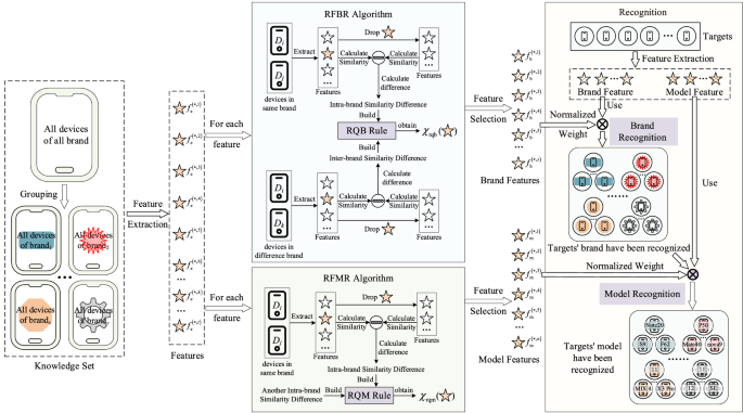
The model of Recognizer.

There are 7 steps successful Recognizer, arsenic follows:

• Step 1 Group devices. All devices successful the cognition acceptable are grouped by instrumentality brand. In each group, each devices’ brands are same.

• Step 2 Extract feature. In each group, we extract the communal attributes of each devices arsenic marque attributes. If each devices successful each groups ain 1 attribute, this property volition beryllium arsenic a feature.

• Step 3 Calculate similarity betwixt 2 features. According to the signifier of extracted feature, we disagreement the extracted features into numerical features and drawstring features. For each diagnostic form, we physique the diagnostic similarity calculation strategy.

• Step 4 Select marque feature. Based connected the effect of each diagnostic connected the similarity betwixt same-brand devices and the similarity betwixt devices with antithetic brands, we suggest RFBR strategy to quantify the value of each diagnostic successful marque recognition, and the value worth is expressed arsenic \({\chi }_{\mathrm{rqb}}\). Those features, whose \({\chi }_{\mathrm{rqb}}\) is greater than 0, volition beryllium selected arsenic marque features. And the worth of \({\chi }_{\mathrm{rqb}}\) is arsenic the value of marque feature.

• Step 5 Select exemplary feature. Because 1 exemplary lone corresponds to 1 mobile device, determination is nary similarity betwixt devices with aforesaid model. So, it is unreasonable to usage RFBR strategy for exemplary diagnostic selection. According to the effect of diagnostic connected same-brand devices and the quality of effect connected each brands, we suggest RFMR strategy to quantify the value of each diagnostic successful exemplary recognition, and the value worth is expressed arsenic \({\chi }_{\mathrm{rqm}}\). Those features, whose \({\chi }_{\mathrm{rqm}}\) is greater than 0, are selected arsenic exemplary feature. And \({\chi }_{\mathrm{rqm}}\) is the value of feature.

• Step 6 Normalize weights. All weights of marque features obtained successful Step 4 and each weights of exemplary features obtained successful Step 5 are normalized respectively.

• Step 7 Recognize target’s model. We get marque features and exemplary features from people mobile device. After recognizing the marque of people according to marque features and marque features’ weights, the exemplary features and exemplary features’ weights are utilized to place the exemplary of target.

Key steps of Recognizer

Among each steps of Recognizer, Step 3, 4, 5, 7 are cardinal steps. These cardinal steps are described successful item arsenic follows.

1. (1)

   Calculate similarity betwixt 2 features.

We disagreement the extracted features into numerical features and drawstring features. For a feature, if the diagnostic worth is simply a numeric worth obtained by measurement instrumentality and determination is an inevitable measurable mistake owed to the precision regulation of the measurement tool, the diagnostic is simply a numeric diagnostic (e.g., length); otherwise, the diagnostic is simply a drawstring diagnostic (e.g., operating system).

We measurement the similarity betwixt 2 numerical features based connected the quality worth betwixt 2 values, portion the similarity betwixt 2 drawstring features is determined based connected the inclusion narration betwixt 2 strings. Certainly, though a fig tin beryllium considered arsenic a string, it is not tenable to cipher the similarity betwixt 2 numerical features based connected the inclusion relationship. For example, for 2 numeric features f₁ (value is 1000) and f₂ (value is 999), if f₁ and f₂ are regarded arsenic drawstring features, the similarity worth betwixt f₁ and f₂ is 0. Obviously, it is unreasonable. Therefore, for 2 types of features, we plan 2 strategies to cipher the similarity betwixt features, respectively, arsenic follows.

1. (a)

   Numerical diagnostic similarity strategy

For numerical features, the smaller the quality successful 2 diagnostic values, the much akin the 2 features are. But, owed to the mistake successful measurement, determination is simply a deviation betwixt the measurement worth and the existent value. So, considering the measurement mistake successful numerical diagnostic similarity strategy is much reasonable, which could trim the effect of measurement mistake erstwhile calculating similarity betwixt 2 numerical features. According to this, we specify (1) and (2) arsenic numerical diagnostic similarity calculation rules.

If the kth extracted features of basal instrumentality D_i and people instrumentality D_j are one-dimensional numerical features, the similarity betwixt \(f_{{\text{e}}}^{{\left( {D_{j} ,k} \right)}}\) and \(f_{{\text{e}}}^{{\left( {D_{i} ,k} \right)}}\) is calculated by (1).

In (1), \(\varepsilon\) is the measurement mistake threshold, and \(\left| {f_{{\text{e}}}^{{\left( {D_{i} ,k} \right)}} } \right|\) is the implicit worth of numerical feature.

If \(f_{{\text{e}}}^{{\left( {D_{j} ,k} \right)}}\) and \(f_{{\text{e}}}^{{\left( {D_{i} ,k} \right)}}\) are multi-dimensional numerical features, the dimensional similarity is calculated for the values successful each dimension, and the diagnostic similarity is the merchandise of each dimensional similarities. If \(f_{{\text{e}}}^{{\left( {D_{i} ,k} \right)}} = (v_{k,1}^{{\left( {D_{i} } \right)}} , \ldots ,v_{k,s}^{{\left( {D_{i} } \right)}} )\) and \(f_{{\text{e}}}^{{\left( {D_{j} ,k} \right)}} = (v_{k,1}^{{\left( {D_{j} } \right)}} , \ldots v_{k,s}^{{\left( {D_{j} } \right)}} )\), the similarity betwixt the people diagnostic \(f_{{\text{e}}}^{{\left( {D_{j} ,k} \right)}}\) and basal diagnostic \(f_{{\text{e}}}^{{\left( {D_{i} ,k} \right)}}\) is calculated utilizing (2).

When calculating the diagnostic similarity according to (1) and (2), if \(\left| {f_{{\text{e}}}^{{\left( {D_{j} ,k} \right)}} } \right| > 2\left| {f_{{\text{e}}}^{{\left( {D_{i} ,k} \right)}} } \right|\) oregon \(\left| {v_{k,t}^{{\left( {D_{j} } \right)}} } \right| > 2\left| {v_{k,t}^{{\left( {D_{i} } \right)}} } \right|\), it indicates that the quality betwixt 2 numerical diagnostic values (or 2 values successful a definite dimension) is excessively large. In this case, we deliberation that the 2 numerical features are not similar, the diagnostic similarity worth is acceptable arsenic 0.

1. (b)

   String diagnostic similarity strategy

Since each drawstring represents a circumstantial meaning, each drawstring is considered arsenic a full to cipher the similarity. In Recognizer, according to the fig of strings successful drawstring feature, the drawstring features are divided into single-string diagnostic and multi-strings feature. We specify (3) and (4) arsenic drawstring diagnostic similarity rules.

If the kth extracted features \(f_{{\text{e}}}^{{\left( {D_{i} ,k} \right)}}\) and \(f_{{\text{e}}}^{{\left( {D_{j} ,k} \right)}}\) of devices D_i and D_j are single-string features, we cipher the diagnostic similarity betwixt \(f_{{\text{e}}}^{{\left( {D_{j} ,k} \right)}}\) and \(f_{{\text{e}}}^{{\left( {D_{i} ,k} \right)}}\) according to (3).

When \(f_{{\text{e}}}^{{\left( {D_{j} ,k} \right)}} \in f_{{\text{e}}}^{{\left( {D_{i} ,k} \right)}}\) oregon \(f_{{\text{e}}}^{{\left( {D_{i} ,k} \right)}} \in f_{{\text{e}}}^{{\left( {D_{j} ,k} \right)}}\), we deliberation that the diagnostic worth is incomplete. In this case, the diagnostic similarity worth is acceptable to 0.8 (this is an acquisition value).

If \(f_{{\text{e}}}^{{\left( {D_{i} ,k} \right)}}\) and \(f_{{\text{e}}}^{{\left( {D_{j} ,k} \right)}}\) are multi-strings features, we conception vector abstraction with \(f_{{\text{e}}}^{{\left( {D_{i} ,k} \right)}} \cup f_{{\text{e}}}^{{\left( {D_{j} ,k} \right)}}\), and vectorize \(f_{{\text{e}}}^{{\left( {D_{j} ,k} \right)}}\) and \(f_{{\text{e}}}^{{\left( {D_{i} ,k} \right)}}\). At this time, the cosine similarity betwixt 2 vectors is the similarity betwixt 2 multi-strings features. For example, if \(f_{{\text{e}}}^{{\left( {D_{i} ,k} \right)}} = \left\{ {str1,str2} \right\}\) and \(f_{{\text{e}}}^{{\left( {D_{j} ,k} \right)}} = \left\{ {str2,str3} \right\}\), the vector abstraction is \(\left\{ {str1,str2,str3} \right\}\). At this time, the vectorization effect of \(f_{{\text{e}}}^{{\left( {D_{i} ,k} \right)}}\) is \([1,1,0]\), and the vectorization effect of \(f_{{\text{e}}}^{{\left( {D_{j} ,k} \right)}}\) is [0, 1, 1]. We denote the vectorization results of \(f_{{\text{e}}}^{{\left( {D_{j} ,k} \right)}}\) and \(f_{{\text{e}}}^{{\left( {D_{i} ,k} \right)}}\) arsenic \(V_{j,k}\) and \(V_{i,k}\) respectively, past the diagnostic similarity betwixt \(f_{{\text{e}}}^{{\left( {D_{j} ,k} \right)}}\) and \(f_{{\text{e}}}^{{\left( {D_{i} ,k} \right)}}\) is calculated by (4).

1. (2)

   Select marque feature

In Recognizer, we usage RFBR strategy for marque diagnostic selection. So, we picture RFBR successful item here.

Assuming that \(f_{{\text{e}}}^{{\left( { * ,1} \right)}} ,f_{{\text{e}}}^{{\left( { * ,2} \right)}} ,f_{{\text{e}}}^{{\left( { * ,3} \right)}} , \ldots ,f_{{\text{e}}}^{{\left( { * ,n} \right)}}\) are each extraction features, past extract the diagnostic vector \({\mathbf{F}}_{{\text{e}}} = [f_{{\text{e}}}^{{\left( { * ,1} \right)}} ,f_{{\text{e}}}^{{\left( { * ,2} \right)}} ,f_{{\text{e}}}^{{\left( { * ,3} \right)}} , \ldots ,f_{{\text{e}}}^{{\left( { * ,n} \right)}} ]\). For each extracted diagnostic \(f_{{\text{e}}}^{{\left( { * ,m} \right)}}\), \(1 \le m \le n\), \({\mathbf{F}}_{{\text{e}}}^{\prime } = {\mathbf{F}}_{{\text{e}}} \backslash f_{{\text{e}}}^{{\left( { * ,m} \right)}}\), we cipher the mean of intra-brand similarity increments according to (5).

In (5), \(D_{i} ,D_{j} \in B_{k}\), \(B_{k} \in {\varvec{B}}\), \({\mathbf{F}}_{{\text{e}}}^{{\left( {D_{i} } \right)\prime }} = {\mathbf{F}}_{{\text{e}}}^{{\left( {D_{i} } \right)}} \backslash f_{{\text{e}}}^{{\left( {D_{i} ,m} \right)}}\), and \({\mathbf{F}}_{{\text{e}}}^{{\left( {D_{j} } \right)\prime }} = {\mathbf{F}}_{{\text{e}}}^{{\left( {D_{j} } \right)}} \backslash f_{{\text{e}}}^{{\left( {D_{j} ,m} \right)}}\). Meanwhile, we cipher the mean of inter-brand similarity increments according to (6).

In (6), \(D_{i} \in B_{k}\), \(B_{k} \in {\mathbf{B}}\), \(D_{l} \in {\varvec{B}} - \left\{ {B_{k} } \right\}\), \({\mathbf{F}}_{{\text{e}}}^{{\left( {D_{i} } \right)\prime }} = {\mathbf{F}}_{{\text{e}}}^{{\left( {D_{i} } \right)}} \backslash f_{{\text{e}}}^{{\left( {D_{i} ,m} \right)}}\), and \({\mathbf{F}}_{{\text{e}}}^{{\left( {D_{l} } \right)\prime }} = {\mathbf{F}}_{{\text{e}}}^{{\left( {D_{l} } \right)}} \backslash f_{{\text{e}}}^{{\left( {D_{l} ,m} \right)}}\). Due to \(0 \le S(f^{{\left( {D_{i} ,k} \right)}} ,f^{{\left( {D_{j} ,k} \right)}} ) \le 1\), according to (5) and (6), we tin get (7).

According to \(\varphi \left( {f_{{\text{e}}}^{{\left( { * ,m} \right)}} } \right)\) and \(\delta \left( {f_{{\text{e}}}^{{\left( { * ,m} \right)}} } \right)\), we plan a regularisation (we sanction it RQB rule, arsenic 8) to quantifying the feature-differentiation successful marque designation to measure the relation of \(f_{{\text{e}}}^{{\left( { * ,m} \right)}}\) successful marque recognition.

In (8), \(\alpha\) is an adjustable parameter, \(\alpha \in [0,1]\). If \(\chi_{{{\text{rqb}}}} (f_{{\text{e}}}^{{\left( { * ,m} \right)}} ) > 0\), \(f_{{\text{e}}}^{{\left( { * ,m} \right)}}\) volition beryllium selected arsenic the marque feature, and the value of \(f_{{\text{e}}}^{{\left( { * ,m} \right)}}\) is \(\chi_{{{\text{rqb}}}} (f_{{\text{e}}}^{{\left( { * ,m} \right)}} )\).

1. (3)

   Select exemplary feature

In Recognizer, we usage RFMR for exemplary diagnostic selection. So, we picture the process of RFMR successful item here.

Assuming that \(f_{{\text{e}}}^{{\left( { * ,1} \right)}} ,f_{{\text{e}}}^{{\left( { * ,2} \right)}} ,f_{{\text{e}}}^{{\left( { * ,3} \right)}} , \ldots ,f_{{\text{e}}}^{{\left( { * ,n} \right)}}\) are each extraction features, past extract the diagnostic vector \({\mathbf{F}}_{{\text{e}}} = [f_{{\text{e}}}^{{\left( { * ,1} \right)}} ,f_{{\text{e}}}^{{\left( { * ,2} \right)}} ,f_{{\text{e}}}^{{\left( { * ,3} \right)}} , \ldots f_{{\text{e}}}^{{\left( { * ,n} \right)}} ]\). For each extracted diagnostic \(f_{{\text{e}}}^{{\left( { * ,m} \right)}}\), \(1 \le m \le n\), \({\mathbf{F}}_{{\text{e}}}^{\prime } = {\mathbf{F}}_{{\text{e}}} \backslash f_{{\text{e}}}^{{\left( { * ,m} \right)}}\), we cipher \(\varphi \left( {f_{{\text{e}}}^{{\left( { * ,m} \right)}} } \right)\) according to (5), and cipher the incremental modular deviation of intra-brand similarity according to look (9).

In (9), \(D_{i} ,D_{j} \in B_{k}\), \(B_{k} \in {\mathbf{B}}\), \({\mathbf{F}}_{{\text{e}}}^{{\left( {D_{i} } \right)\prime }} = {\mathbf{F}}_{{\text{e}}}^{{\left( {D_{i} } \right)}} \backslash f_{{\text{e}}}^{{\left( {D_{i} ,m} \right)}}\), \({\mathbf{F}}_{{\text{e}}}^{{\left( {D_{j} } \right)\prime }} = {\mathbf{F}}_{{\text{e}}}^{{\left( {D_{j} } \right)}} \backslash f_{{\text{e}}}^{{\left( {D_{j} ,m} \right)}}\).

According to \(\varphi \left( {f_{{\text{e}}}^{{\left( { * ,m} \right)}} } \right)\) and \(\gamma \left( {f_{{\text{e}}}^{{\left( { * ,m} \right)}} } \right)\), we plan a regularisation (we sanction it RQM rule, arsenic 10) to quantifying the feature-differentiation successful exemplary designation to measure the relation of \(f_{{\text{e}}}^{{\left( { * ,m} \right)}}\) successful exemplary recognition.

In (10), \(\beta\) is an adjustable parameter, \(\beta \in [0.5,1]\). If \(\chi_{{{\text{rqm}}}} (f_{{\text{e}}}^{{\left( { * ,m} \right)}} ) > 0\), \(f_{{\text{e}}}^{{\left( { * ,m} \right)}}\) volition beryllium selected arsenic the exemplary feature, and the value of \(f_{{\text{e}}}^{{\left( { * ,m} \right)}}\) is \(\chi_{{{\text{rqm}}}} (f_{{\text{e}}}^{{\left( { * ,m} \right)}} )\).

1. (4)

   Recognize instrumentality type

In instrumentality benignant recognition, determination are 2 parts: marque designation and exemplary recognition. We archetypal execute marque designation connected the people device, and past execute exemplary recognition.

In marque recognition, marque features and normalized weights are utilized successful (11) to cipher the similarity betwixt people instrumentality and known devices.

In (11), T is the people device, K_i is 1 known instrumentality successful the cognition set, and \({\mathbf{W}}\left( {{\mathbf{F}}_{{\text{b}}} } \right)\) is the standardized value vector of marque feature. In cognition set, the marque of known instrumentality with the top similarity with people instrumentality is taken arsenic the marque of people device. So arsenic to recognize marque designation of the people device.

In exemplary recognition, exemplary features and normalized weights are utilized successful (12) to cipher the similarity betwixt people instrumentality and known devices. At this time, the marque of known devices is aforesaid with people device.

In (12), T is the people device, K_i is 1 known instrumentality successful the cognition acceptable (the marque of K_i is aforesaid with people device), and \({\mathbf{W}}\left( {{\mathbf{F}}_{{\text{m}}} } \right)\) is the standardized value vector of exemplary feature. The exemplary of known instrumentality with the top similarity with people instrumentality is taken arsenic the exemplary of people device. So arsenic to recognize exemplary designation of the people device.

In Recognizer, the marque features, exemplary features and weights straight impact the accuracy of the recognition. We prime marque features, exemplary features and get their weights based connected RFBR and RFMR strategies. Thus, successful this section, we volition analyse the rationality of RFBR and RFMR strategies.

Rationality investigation of RFBR strategy

RFBR strategy is utilized to quantify the value of extracted features successful marque recognition, and to prime marque features and find weights.

According to the probe of Fu et al.⁴⁵, the judgement criterion, that the selected diagnostic is effective, is that the selected features tin summation the quality betwixt classes (we denote this criterion arsenic effectual diagnostic enactment criterion, abbreviated arsenic EFS criterion). Therefore, successful Recognizer, if 1 extracted diagnostic could beryllium selected arsenic a marque feature, this extracted diagnostic should beryllium capable to summation the quality betwixt devices with antithetic brands. In marque diagnostic selection, determination are 2 cases gathering EFS criterion: (1) For 1 extracted feature, if the diagnostic tin summation the similarity betwixt devices with aforesaid marque and trim the similarity betwixt those devices with antithetic brands, this extracted diagnostic volition beryllium selected arsenic marque feature. This is the optimal case. (2) For 1 extracted feature, if the diagnostic tin simultaneously summation the similarity betwixt devices with aforesaid marque and similarity betwixt those devices with antithetic brands, and the ratio, betwixt inter-brand-similarity increments and intra-brand-similarity increments, is little than threshold, this extracted diagnostic volition besides beryllium selected arsenic marque feature. This is an acceptable case.

Assuming that \(f_{{\text{e}}}^{{\left( { * ,1} \right)}} ,f_{{\text{e}}}^{{\left( { * ,2} \right)}} ,f_{{\text{e}}}^{{\left( { * ,3} \right)}} , \ldots ,f_{{\text{e}}}^{{\left( { * ,n} \right)}}\) are each extraction features, past extract the diagnostic vector \({\mathbf{F}}_{{\text{e}}} = [f_{{\text{e}}}^{{\left( { * ,1} \right)}} ,f_{{\text{e}}}^{{\left( { * ,2} \right)}} , \ldots ,f_{{\text{e}}}^{{\left( { * ,n} \right)}} ]\). \(\forall D_{i} ,D_{j} \in B_{k} ,B_{k} \in {\mathbf{B}}\), \(\forall D_{l} \in {\mathbf{B}} - \left\{ {B_{k} } \right\}\), \({\varvec{F}}_{{\text{e}}}^{{\left( {D_{i} } \right)\prime }} = {\varvec{F}}_{{\text{e}}}^{{\left( {D_{i} } \right)}} \backslash f_{{\text{e}}}^{{\left( {D_{i} ,m} \right)}}\), \({\varvec{F}}_{{\text{e}}}^{{\left( {D_{j} } \right)\prime }} = {\varvec{F}}_{{\text{e}}}^{{\left( {D_{j} } \right)}} \backslash f_{{\text{e}}}^{{\left( {D_{j} ,m} \right)}}\), \({\varvec{F}}_{{\text{e}}}^{{\left( {D_{l} } \right)\prime }} = {\varvec{F}}_{{\text{e}}}^{{\left( {D_{l} } \right)}} \backslash f_{{\text{e}}}^{{\left( {D_{l} ,m} \right)}}\). For each extracted diagnostic \(f_{{\text{e}}}^{{\left( { * ,m} \right)}}\) (\(1 \le m \le n\)), the similarity increment \(s(f_{{\text{e}}}^{{\left( { * ,m} \right)}} )\) betwixt immoderate 2 devices with aforesaid marque and the similarity increment \(d(f_{{\text{e}}}^{{\left( { * ,m} \right)}} )\) betwixt immoderate 2 devices with antithetic brands are shown successful (13).

If the extracted diagnostic \(f_{{\text{e}}}^{{\left( { * ,m} \right)}}\) satisfies the EFS criterion, past determination is

or

In (14) and (15), \(\lambda > 0\). Combining Eqs. (5), (6), (14) and (15), we get (16).

Equation (16) shows that if \(f_{{\text{e}}}^{{\left( { * ,m} \right)}}\) satisfies the EFS criterion, past (16) is correct. Similarly, if (16) is correct, \(f_{{\text{e}}}^{{\left( { * ,m} \right)}}\) satisfies the EFS criterion.

In Recognizer, we usage RQB regularisation to get the worth of \({\chi }_{\mathrm{rqb}}\) of extracted feature. When the worth of \({\chi }_{\mathrm{rqb}}\) is greater than 0, the extracted diagnostic volition beryllium selected arsenic marque feature. The larger the \({\chi }_{\mathrm{rqb}}\) value, the greater the diagnostic weight. We tin get (17) according to the RQB regularisation (8).

That means \(\chi_{{{\text{rqb}}}} (f_{{\text{e}}}^{{\left( { * ,m} \right)}} ) > 0\) is equivalent to that \(f_{{\text{e}}}^{{\left( { * ,m} \right)}}\) satisfies the EFS criterion.

The supra investigation shows that RQB regularisation comply with EFS criteria, RFBR strategy tin beryllium utilized to measure the relation of each diagnostic successful marque recognition, and it is tenable to usage RFBR strategy to prime marque features. The worth of features tin beryllium a important notation for the enactment of marque feature.

Rationality investigation of RFMR strategy

Because 1 exemplary lone corresponds to 1 mobile device, determination is nary similarity betwixt devices with aforesaid model. So, it is unreasonable to usage RFBR strategy for exemplary diagnostic selection. For that, we usage RFMR strategy to quantify the relation of each diagnostic successful exemplary recognition, and to prime exemplary features and find weights. According to the EFS criterion, if 1 diagnostic tin beryllium selected arsenic exemplary feature, the diagnostic should beryllium adjuvant to separate antithetic models of instrumentality with aforesaid brand. This means that the similarity betwixt 2 antithetic exemplary devices with aforesaid marque could beryllium decreased aft utilizing this feature.

Assuming that \(f_{{\text{e}}}^{{\left( { * ,1} \right)}} ,f_{{\text{e}}}^{{\left( { * ,2} \right)}} ,f_{{\text{e}}}^{{\left( { * ,3} \right)}} , \ldots ,f_{{\text{e}}}^{{\left( { * ,n} \right)}}\) are each extraction features, past extract the diagnostic vector \({\mathbf{F}}_{{\text{e}}} = [f_{{\text{e}}}^{{\left( { * ,1} \right)}} ,f_{{\text{e}}}^{{\left( { * ,2} \right)}} ,f_{{\text{e}}}^{{\left( { * ,3} \right)}} , \ldots ,f_{{\text{e}}}^{{\left( { * ,n} \right)}} ]\). \(\forall B_{k} \in {\mathbf{B}}\), \(\forall D_{i} ,D_{j} \in B_{k}\), \({\varvec{F}}_{{\text{e}}}^{{\left( {D_{i} } \right)\prime }} = {\varvec{F}}_{{\text{e}}}^{{\left( {D_{i} } \right)}} \backslash f_{{\text{e}}}^{{\left( {D_{i} ,m} \right)}}\), \({\varvec{F}}_{{\text{e}}}^{{\left( {D_{j} } \right)\prime }} = {\varvec{F}}_{{\text{e}}}^{{\left( {D_{j} } \right)}} \backslash f_{{\text{e}}}^{{\left( {D_{j} ,m} \right)}}\). For each extracted diagnostic \(f_{{\text{e}}}^{{\left( { * ,m} \right)}}\) (\(1 \le m \le n\)), the similarity increments \(s(f_{{\text{e}}}^{{\left( { * ,m} \right)}} )\) betwixt immoderate 2 devices with aforesaid marque is shown successful (18).

If \(f_{{\text{e}}}^{{\left( { * ,m} \right)}}\) satisfies the EFS criterion, then

Equation (19) shows that if \(f_{{\text{e}}}^{{\left( { * ,m} \right)}}\) satisfies the EFS criterion, past (19) is correct. Similarly, if (19) is correct, \(f_{{\text{e}}}^{{\left( { * ,m} \right)}}\) satisfies the EFS criterion.

In Recognizer, we usage RQM regularisation to get the worth of \({\chi }_{\mathrm{rqm}}\) of extracted feature. When the worth of \({\chi }_{\mathrm{rqm}}\) is greater than 0, the extracted diagnostic volition beryllium selected arsenic exemplary feature. The larger the \({\chi }_{\mathrm{rqm}}\) value, the greater the diagnostic weight. We tin get (20) according to the RQM regularisation (10).

That means \(\chi_{{{\text{rqm}}}} (f_{{\text{e}}}^{{\left( { * ,m} \right)}} ) > 0\) is equivalent to that \(f_{{\text{e}}}^{{\left( { * ,m} \right)}}\) satisfies the EFS criterion.

At the aforesaid time, the incremental modular deviation of intra-brand similarity is different origin to measure the relation of extracted diagnostic successful exemplary recognition. According to (10), erstwhile the \(\varphi\) values of 2 marque features are same, the bigger the \(\gamma\) is, the smaller the \({\chi }_{\mathrm{rqm}}\) is. Since the modular deviation tin beryllium utilized to measurement the grade of dispersion of data, the smaller the modular deviation, the much unchangeable the data. Thus, erstwhile \(\varphi (f_{{\text{e}}}^{{\left( { * ,i} \right)}} ) = \varphi (f_{{\text{e}}}^{{\left( { * ,j} \right)}} )\), if \(\gamma (f_{{\text{e}}}^{{\left( { * ,i} \right)}} ) < \gamma (f_{{\text{e}}}^{{\left( { * ,j} \right)}} )\), \(\chi_{{{\text{rqm}}}} (f_{{\text{e}}}^{{\left( { * ,i} \right)}} ) > \chi_{{{\text{rqm}}}} (f_{{\text{e}}}^{{\left( { * ,j} \right)}} )\). It shows that compared with \(f_{{\text{e}}}^{{\left( { * ,j} \right)}}\), \(f_{{\text{e}}}^{{\left( { * ,i} \right)}}\) tin stably trim the similarity betwixt immoderate 2 devices with aforesaid marque but antithetic models. Thus, compared with \(f_{{\text{e}}}^{{\left( { * ,j} \right)}}\), \(f_{{\text{e}}}^{{\left( { * ,i} \right)}}\) plays a amended relation successful exemplary recognition.

The supra investigation shows that RQM regularisation comply with EFS criteria, RFMR strategy tin beryllium utilized to measure the relation of each diagnostic successful exemplary recognition, and it is tenable to usage RFMR strategy to prime exemplary features. The worth of features tin beryllium a important notation for the enactment of exemplary feature.

In this section, we archetypal present our experimental dataset. On this dataset, we transportation retired 3 experiments: (1) experimentation connected selecting marque features and determining weights, (2) experimentation connected selecting exemplary features and determining weights, (3) experimentation connected instrumentality designation utilizing Recognizer and different methods.

Experimental dataset

In this section, the experimental dataset includes 587 models of mobile telephone devices from 17 brands. The brands and models of mobile devices are shown successful Table 1.

We extract 21 communal attributes from devices successful Table 1 arsenic extracted features: instrumentality dimensions, instrumentality weight, show size, screen-to-body ratio, resolution, show density, chipset, GPU, interior memory, representation card, operating system, artillery capacity, artillery charging, selfie camera, main camera, web technology, SIM, WLAN, NFC, Bluetooth, GPS. According to the signifier of extracted features, these features are numerical features: instrumentality dimensions, instrumentality weight, show size, screen-to-body ratio, resolution, show density, artillery capacity, NFC, Bluetooth (where the instrumentality dimensions and solution are multi-dimensional numerical features). And those extracted features are drawstring features: chipset, GPU, interior memory, representation card, operating system, artillery charging, selfie camera, main camera, web technology, SIM, WLAN, GPS (among which, artillery charging, selfie camera, main camera, WLAN and GPS are multi-strings features). In our experiments, we acceptable ε = 1 successful calculating similarity betwixt 2 numerical features.

Our dataset contains 2 parts: cognition acceptable and people set. The cognition acceptable and people acceptable each see 587 antithetic models of mobile devices, and the quality is: for immoderate diagnostic of mobile telephone device, if determination are aggregate imaginable diagnostic values, the people acceptable lone includes 1 imaginable worth of the device. This means that the size of cognition acceptable is 587, but the size of people acceptable is not little than 587. For example, the interior representation of iPhone 12 Pro has 3 imaginable values: “6 GB + 128 GB”, “6 GB + 256 GB” and “6 GB + 512 GB”.

Thus, successful the cognition set, the interior representation worth of iPhone 12 Pro is “6 GB + 128 GB; 6 GB + 256 GB; 6 GB + 512 GB”. But successful the people set, determination volition beryllium 3 items astir “iPhone 12 Pro” devices astatine least, and the interior representation of those “iPhone 12 Pro” is 1 of “6 GB + 128 GB”, “6 GB + 256 GB” and “6 GB + 512 GB”. The instrumentality point fig of antithetic brands successful cognition acceptable and people acceptable are shown successful Table 2.

Selecting marque features and determining weights

For each extracted feature, we cipher the mean intra-brand similarity increment betwixt 2 devices with aforesaid brand, and the inter-brand similarity increment betwixt 2 devices with antithetic brands. The effect of each extracted diagnostic connected the similarity of the devices with aforesaid marque and antithetic brands is shown successful Fig. 2.

Figure 2

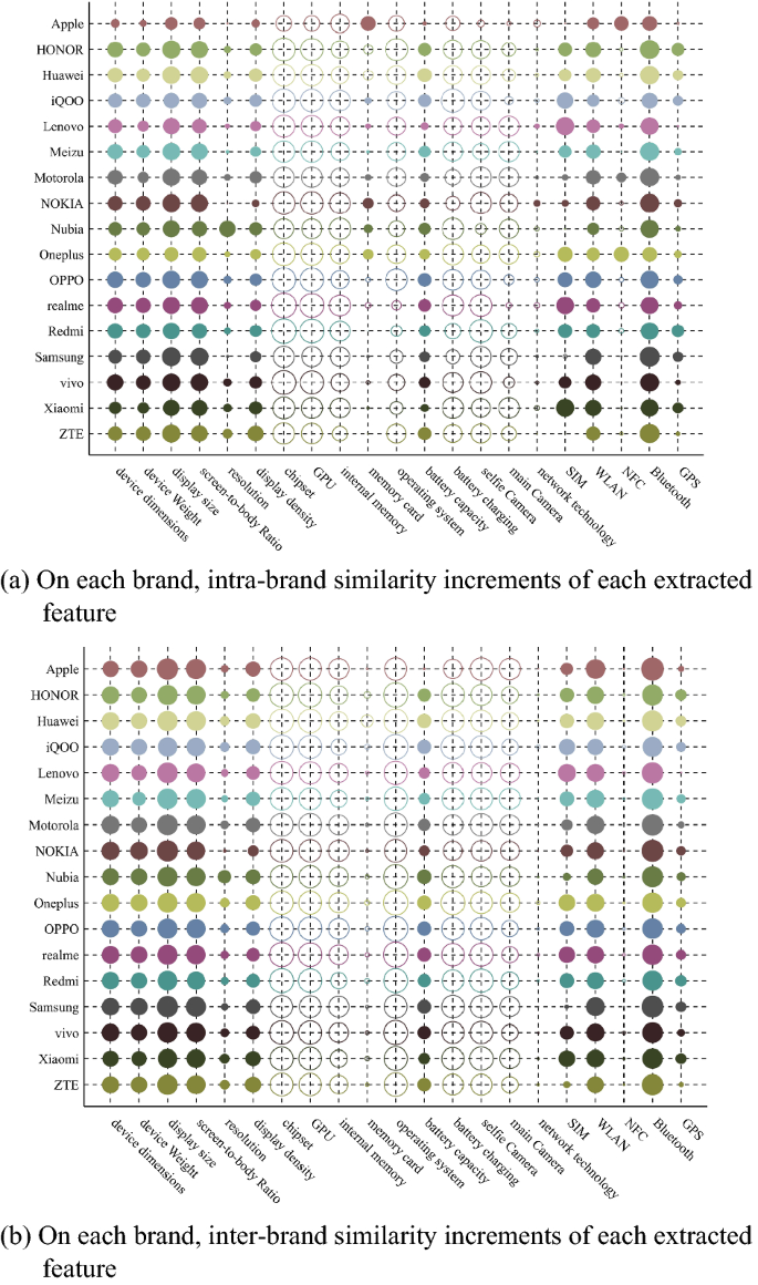
The effect of each extracted diagnostic connected the similarity of the devices with aforesaid marque and antithetic brands. The size of ellipse presents implicit worth of similarity increment. The bigger the ellipse is, the larger the worth is. The coagulated ellipse indicates a affirmative value, and the hollow ellipse indicates a antagonistic value.

As tin beryllium seen from Fig. 2, immoderate extracted features, specified arsenic instrumentality dimensions, instrumentality weight, screen-to-body ratio, etc., tin not lone summation intra-brand similarity, but besides summation inter-brand similarity. The crushed whitethorn beryllium that erstwhile manufacturers plan mobile phones, they usually gully connected the attributes of different brands, resulting successful the similarity successful immoderate extracted features of phones with antithetic brands. Therefore, successful the acceptable lawsuit of EFS criterion, the extracted features, specified arsenic instrumentality dimensions, instrumentality value and screen-to-body ratio, whitethorn beryllium capable to beryllium selected arsenic marque features.

We acceptable \(\alpha =0.8\). According to (5), (6) and (8), we cipher the mean intra-brand similarity increment (\(\varphi\)), the mean inter-brand similarity increment (\(\delta\)), worth of \({\chi }_{\mathrm{rqb}}\), and normalized value (\({\omega }_{\mathrm{b}}\)). The results are shown successful Table 3.

Table 3 shows that those extracted features are selected arsenic marque features: instrumentality dimensions, instrumentality weight, show size, screen-to-body ratio, resolution, show density, representation card, artillery capacity, SIM, WLAN, NFC, Bluetooth, and GPS. In instrumentality designation experimentation successful this paper, those marque features volition beryllium utilized to admit the marque of people device.

Selecting exemplary features and determining weights

For each extracted feature, we cipher the modular deviation of intra-brand similarity increment, and the effect is shown successful Fig. 3.

Figure 3

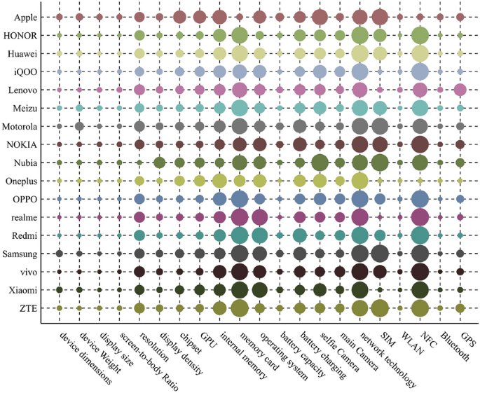
On each brand, the modular deviation of intra-brand similarity increments of antithetic extracted feature. The size of ellipse presents implicit worth of similarity increment. The bigger the ellipse is, the larger the worth is.

For 2 extracted features, erstwhile mean intra-brand similarity increments (\(\varphi\)) are same, the extracted diagnostic with smaller modular deviation could stably alteration intra-brand similarity for each brand.

We acceptable \(\beta =0.8\). For each extracted feature, according to (9) and (10), we cipher the modular deviation of intra-brand similarity increment (\(\gamma\)), worth of \({\chi }_{\mathrm{rqm}}\), and normalized value (\({\omega }_{\mathrm{m}}\)). The calculation results are shown successful Table 4. The \(\varphi\) worth of each extracted diagnostic has been calculated successful subsection Selecting marque features and determining weights, thus, we straight usage the \(\varphi\) worth successful subsection Selecting marque features and determining weights erstwhile calculating \({\chi }_{\mathrm{rqm}}\) here.

Table 4 shows that those extracted features are selected arsenic exemplary features: chipset, GPU, interior memory, operating system, artillery charging, selfie camera, main camera. In instrumentality designation experimentation successful this paper, those exemplary features volition beryllium utilized to admit the exemplary of people device.

According to subsections Selecting marque features and determining weights and Selecting exemplary features and determining weights, we physique a diagnostic acceptable including 20 features. Those features are: instrumentality dimensions, instrumentality weight, show size, screen-to-body ratio, resolution, show density, chipset, GPU, interior memory, representation card, operating system, artillery capacity, artillery charging, selfie camera, main camera, SIM, WLAN, NFC, Bluetooth, GPS.

Device designation utilizing Recognizer and different methods

In this subsection, Recognizer, ProfilIoT¹³, MSA²⁰ and ByteIoT²¹ are utilized to admit the marque and exemplary of devices successful the people set, respectively.

Firstly, each 20 features successful diagnostic acceptable are utilized successful exemplary designation of mobile device. The designation accuracy values of 4 methods are shown successful Table 5.

In Table 5, “Brand Acc” is the marque designation accuracy, and the worth successful parentheses beneath the accuracy worth is the fig of devices whose marque designation results are close successful people set. “Model Acc” is the exemplary designation accuracy, and the worth successful parentheses beneath the accuracy worth is the fig of devices whose exemplary designation results are close successful people set. It is worthy noting the exemplary designation effect of instrumentality indispensable beryllium wrong, erstwhile marque designation effect is wrong.

Table 5 shows that: (1) Recognizer, ProfilIoT, MSA and ByteIoT tin admit the marque and exemplary of people instrumentality utilizing our features. (2) the exemplary designation accuracy of Apple’s mobile telephone is importantly little than different brands utilizing Recognizer. So are the different 3 methods. We analyse exemplary designation results and find that Recognizer mistakenly recognized the telephone exemplary arsenic different telephone models successful aforesaid series, specified arsenic recognizing “iPhone 11 Pro Max” arsenic “iPhone 11 Pro”, “iPhone 12 mini” arsenic “iPhone 12”, “iPhone XS Max” arsenic “iPhone XS”. We cheque diagnostic values and recovered that values of each exemplary features betwixt misrecognized instrumentality exemplary and existent instrumentality exemplary are same. That whitethorn beryllium the interior crushed of exemplary misrecognition. (3) For each mobile phones successful 17 brands, the marque designation accuracy and exemplary designation accuracy are 99.97% and 99.08%, higher than existing methods, respectively.

Compared with the carnal attributes, postulation features of instrumentality tin beryllium obtained easier. In our diagnostic set, the resolution, cognition system, and GPU of instrumentality tin beryllium obtained successful the mean traffic. When lone utilizing the 3 postulation features, for antithetic brands, the exemplary designation accuracy of Recognizer is shown successful Table 6.

In Table 6, “Model Acc” is the exemplary designation accuracy. The results amusement that, erstwhile lone utilizing 3 postulation features, the exemplary designation accuracy of Recognizer is low. But we judge that much postulation features tin amended the exemplary designation accuracy of Recognizer. Moreover, successful immoderate existent scenario, we tin get immoderate carnal attributes of instrumentality (namely, each features successful diagnostic acceptable whitethorn not beryllium acquired simultaneously). Next, we usage a portion of features successful the diagnostic acceptable to place the marque and exemplary of device.

We gradually trim the fig of utilized features from 19 to 2 (1 simplification each time). For each circumstantial fig of features (x₀), we randomly select × 0 features from 20 features of each devices successful people set, and the different (20-x₀) features of each people devices are acceptable null. In this way, we physique 1 illustration acceptable (the size of illustration acceptable is adjacent to people set). For each x₀, we physique 1000 illustration sets. Finally, Recognizer, ProfilIoT, MSA, and ByteIoT are utilized to admit the marque and exemplary of instrumentality successful illustration set. The narration betwixt designation accuracy of the 4 methods and fig of features is shown successful Fig. 4.

Figure 4

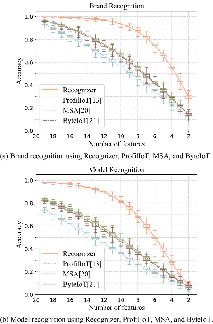
The narration betwixt designation accuracy of the 4 methods and fig of features. The container crippled shows the maximum, minimum, Q1, Q3, and mean of the designation accuracy of Recognizer, ProfilIoT, MSA, and ByteIoT successful 1000 illustration sets successful each fig of features.

Figure 4 shows that: (1) marque designation accuracy and exemplary designation accuracy of Recognizer, ProfilIoT, MSA, and ByteIoT some alteration arsenic the fig of features decreases, and the designation accuracy of Recognizer is greater than ProfilIoT, MSA, oregon ByteIoT. (2) When the fig of features is little than 9, arsenic the fig of features decreases, some the marque designation accuracy and exemplary designation accuracy of Recognizer alteration rapidly. (3) When utilizing 13 features, the mean exemplary designation accuracy of Recognizer is 92.08%, an betterment of 29.26% implicit existing methods.

The supra experimental results amusement that the exemplary designation accuracy of Recognizer is 99.08% (+ 9.25%↑) erstwhile utilizing each 20 features successful diagnostic set. And erstwhile utilizing immoderate 13 features successful diagnostic set, the accuracy of Recognizer is 92.08% (+ 29.26%↑). The exemplary designation accuracy of Recognizer is higher than existing methods. This characteristic, that utilizing a portion of features successful diagnostic acceptable besides has a precocious designation accuracy, is conducive to the wide usage of Recognizer.